How To Set Up A Budget In Google Sheets

Information technology probably won't surprise you to hear that I employ a Google Sheets budget template to track my finances, both incomings and approachable, at domicile and for my business.

The dashboards bachelor through online banking sites are pretty rudimentary. They don't give much insight into what'southward happening with my finances, particularly over longer time frames.

I like using Google Sheets, as opposed to another third political party service similar Mint, considering it's fully customizable. It's easy to apply and I can share any spending or budget templates easily with my married woman.

I'thousand not a financial skillful, so I won't be dispensing any financial communication hither. I won't opine on what you should or shouldn't testify in your spending and budget templates in this post, nor will I talk nearly what your financial goals should be or how to get in that location.

What I will practice in this post all the same, is show yous some useful tips in Google Sheets that you can utilise for edifice your own upkeep templates. Techniques to make them more than insightful and more helpful for reaching your goals.

Here's a summary of what we'll comprehend for edifice a Google Sheets budget template:

1. Earlier you lot build, consider your why
2. Invest fourth dimension piddling and frequently
3. Go basic formulas dialed
4. Leverage power of more avant-garde formulas
5. Don't reinvent the cycle! Google has specific financial formulas
6. Use comments to record specific details
7. Import your financial data into Google Sheets with Tiller
8. Set up budgets and highlight spend over the budgeted amount
9. Build drop-downwards menus to show different categories in your reports
10. Use words!

10 tips to build a Google Sheets budget template

Here are x tips for creating a Google Sheets budget template:

1. Earlier you lot build, consider your why

Earlier diving into the thick of it, and getting lost in your transactions, fancy formulas or complex charts, it'south worth spending some time thinking nearly why you're doing this.

Putting bated spreadsheets, and tracking, and expenses for a moment, ask yourself what it is you lot're trying to do (for instance, possibly you want to pay off a student loan equally chop-chop every bit possible, or reduce your credit carte spending each month considering it's as well loftier! ?).

What problem are you lot trying to solve?

And then, gear up a goal!

Work out what would assistance you reach that goal (for instance being able to see how much, and where you spend your money each month). Then build yourself a Google Sail template that will do that for you (for example a Sheet showing your credit bill of fare transactions broken down into different categories).

Don't try to create one giant spreadsheet to rails everything (at least not initially). You'll be meliorate served by creating a single, focused Google Sheet that solves ane problem for you.

Here are some ideas: credit card spending/budget templates, student loan tracker, mortgage payment tracker, stock portfolio tracker, household budget templates, childcare costs,….etc.

two. Invest time, little and often

Ok, so building a template is going to take some time up forepart. Anything from an hr for a basic template, up to mayhap a day or 2 to build something circuitous.

However, once y'all take your template, it'll so simply accept a few minutes each twenty-four hour period to keep on top of things. And that'due south the beauty of this whole procedure.

Speedily update your transactions, tweak your categories, change a chart and, most chiefly of all, empathise and glean insights almost your finances.

The upfront endeavour pays dividends down the line when you have a clear censor knowing what yous're spending and how y'all compare to your budget.

3. Go basic formulas dialed

It goes without maxim that you'll employ the SUM formula in your upkeep templates, and I won't insult your intelligence by covering that.

Y'all'll probably too find yourself using AVERAGE, MIN and MAX, which are again, piece of cake to understand.

Another one you'll probably want to employ in your Google Sheets upkeep template, and one that oftentimes trips people up, is the Percentage alter formula, so allow's run through a quick example of that. The formula is:

(New amount - Original amount) / Original Amount

Take your new value (due east.g. this month) and minus your original value (e.k. last month). Accept this answer (the difference between New and Original) and dissever it by the original amount (due east.g. last month).

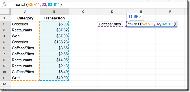
There are other, super-useful, and relatively bones formulas you may not take used before: SUMIF and SUMIFS (and corresponding AVERAGEIF and AVERAGEIFS, aforementioned principle).

The SUMIF part allows you to sum your data, just but when a specific criterion is met. For instance, maybe you want to sum everything in category X, or calendar month Y, or on credit card Z. SUMIF (or SUMIFS) is the formula you'll want to use.

It takes the class:

=SUMIF( range to test, examination criteria, range of values to sum)

So a real example would expect like this, where nosotros exam cavalcade A for "Java/Bites" and only add values from B to the total for rows that friction match:

The SUMIFS part is slightly different, because y'all specify the sum range (i.e. the range of values you want to sum) first, and and so all your different conditions.

iv. Leverage power of more advanced formulas in your Google Sheets upkeep template

In that location are a few other key formulas that are worth investing fourth dimension in. You'll be able to dispense your data more than hands with a mastery of these formulas and brandish it in new ways for a more sophisticated understanding of your finances.

I'd recommend learning the following formulas:

VLOOKUP

The VLOOKUP office is arguably the most famous advanced formula in the spreadsheet world. Give it a search term and information technology volition search for this term in a separate table and render specific data if it finds the search term. It's actually useful for edifice dynamic tables and charts (see section 9 below).

The VLOOKUP can as well exist wrapped in an IFERROR office to handle any errors (if the search term is not establish, you lot can set a custom message to display due east.chiliad. "No information constitute for this month"):

=IFERROR(VLOOKUP($A10,$AF:$AG,2,fake),"No data found for this calendar month")

FILTER

The FILTER function allows you lot to bear witness a subset of data that passes some criteria. For instance, you might want to filter so you but see transactions over $250, when you lot want to easily check all your large transactions. Or maybe filter on all transactions from a sure vendor, to come across how much you've spent with them.

It'due south relatively simple to implement:

=FILTER( range, atmospheric condition we're testing for)

In practice, if we had our data in the range A1:D100, with values in column D, and we wanted to see simply transactions over $250, our formula would exist:

=FILTER( A1:D100, D1:D100 > 250)

QUERY

If you thought the filter office was useful, wait until you acquire how to wield the QUERY part. It's arguably the most powerful office in Google Sheets. Menses.

It tin amass your data, summarize your data, filter your data, sort your data, you name it and it can probably do it. Even so it's not an easy formula to acquire:

=QUERY($A$1:$B,"select A, sum(B) where B > 0 group by A order by A desc characterization A 'Month', sum(B) 'Payments'")

This case takes data in columns A and B and groups on the month in cavalcade A (so all January payments get added together, all Feb payments get added together etc.). Information technology merely includes payments greater than 0. It sorts the months in lodge and relabels the columns of the new Query table equally 'Month' and 'Payments'.

As you lot tin see, it's a very powerful function.

5. Don't reinvent the wheel! Google has specific financial formulas

Google Sheets has over 40 built-in fiscal formulas, for solving very specific needs, everything from depreciation to treasury yields.

And so bank check out the full listing hither, before doing legwork you don't demand to do.

Let'south take a quick look at one of the more general formulas, FV, which calculates the hereafter value based on constant-amount periodic payments and a constant interest charge per unit.

The general formula is:

= FV(rate, number_of_periods, payment_amount, present_value, [end_or_beginning])

I recently used this formula to calculate the future value of a lump sum, invested at a v% return for 30 years. The idea was to show how the corporeality I'd spent over my upkeep could accept been invested instead, and show what it might have been worth in xxx years time. The lost opportunity cost.

And so it's five% interest, divided by 12 to become a monthly rate. Next the number of monthly periods, 360. The payment amount is 0, since I don't want to include any payments. The present value is the spend this month, less my target budget (i.due east. the amount over budget). The last argument, [end_or_beginning], is optional and relates to whether the payments are made at the beginning or end of the month, so non relevant in this case.

=FV(0.05/12,360,,-(C26 - $E$3))

Read more near the FV role in the docs here.

6. Employ comments to record specific details

Oft I find myself wanting to add a annotation to a transaction, because something nearly it is different than normal and I know I'll forget why if I don't write it downwards. However, I don't actually desire to accept to add extra rows or columns, or rebuild my upkeep templates but to fit more than text cells in.

And so I add comments to record specific details nigh a transaction.

You lot can add comments to cells in spreadsheets past right clicking and selecting "Insert comment":

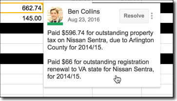
All-time of all, you tin can tag others in a comment to notify them, by typing "@" + their electronic mail address. For example you might tag an unusual looking transaction for your accountant to review.

If you have a lot of context to tape, or find yourself wanting to add together notes every month, then a defended notes cavalcade is the way to get. Simply for occasional notes, comments are the style to go. They're low profile and won't affect any calculations.

7. Import your financial information into Google Sheets with Tiller

You lot'd imagine that building all these templates in Google Sheets would crave us to download our data from the financial vendors, as a CSV file we could import into Google Sheets.

Non so!

I use an amazing tool called Tiller to bring all my financial information into my Google Sheets, so I can analyze it and build templates exactly equally I want.

It's my underground weapon for edifice fiscal templates.

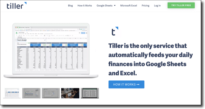
You tin can use Tiller to bring depository financial institution account information, credit card data, or other financial data into your Google Sheets. Information technology's super easy to setup and works flawlessly for me.

The data is updated every forenoon when y'all'll also receive an email summary update:

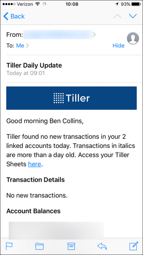
It costs $79/year, which is tremendous value since you lot're getting a fully customizable, automated personal finance tool.

8. Fix budgets and highlight spend over the budgeted corporeality

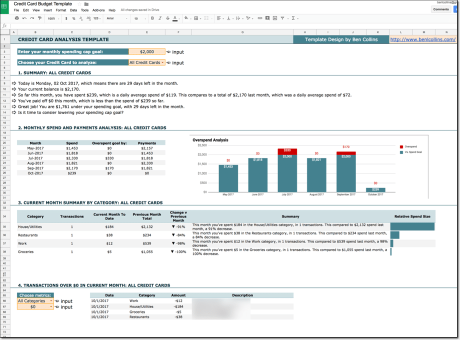
The following chart shows any spend over $2,000 in a calendar month with a red color, to differentiate it and bring it to the attending of the viewer. It's a classic technique in data visualization, using a pre-circumspect aspect to convey information more finer.

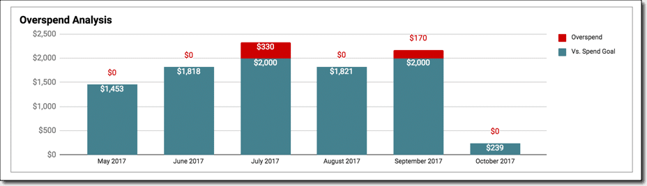
It's easy to exercise in Google Sheets. You lot can apply simple formulas to split up amounts above the threshold and then turn your regular column chart into a stacked column chart.

The table is simply two columns. The offset shows the value or the threshold, whichever is smaller. The 2nd shows a 0, unless the value is over the threshold, in which example it displays the difference.

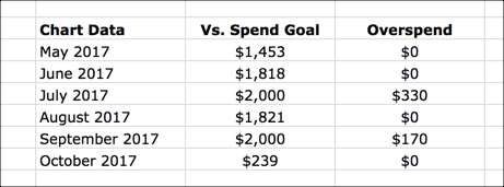
Assuming my threshold value of $2,000 is in cell E3, and my column of spend values is column C, the formulas are:

=MIN( C21, $E$3 )

and

=IF( C21 > $Due east$iii, C21 - $Due east$iii, 0 )

9. Build driblet-downward menus to bear witness different categories in your Google Sheets upkeep template

It's really easy to add category menus in Google Sheets, using Information Validation to build dropdown lists. Then you can change what information is showing in your reports.

These are the steps to create a dynamic chart in your reports:

• Categorize transactions into meaningful groups (similar Groceries, Utilities, Car payments, Mortgage, Discretionary, Restaurants etc.)
• Create a unique list of the category names
• Choose the cell where you want to add together the menu, right click and choose Data Validation...
• Choose "List from range" as the criteria
• Select the unique listing of categories
• Utilise a lookup formula (VLOOKUP) with this information validation prison cell as the search term
• Use the dynamic data table for your chart
• Voila! Your chart will be dynamic too

I've written extensively well-nigh dynamic charts in this post, so I won't repeat it here.

10. Use words!

Peradventure the near influential dashboard article I've ever read is this one from Google Analytics advocate Avinash Kaushik. The takeaway is to include more context and more text in our dashboards, so they reach their potential as determination-making tools, rather than pure "data pukes".

I always keep this in listen when I'yard producing dashboard reports.

For example, in the credit carte du jour template I've shown you, I kickoff with a list of bullet points, which gives me a really good overview of the calendar month:

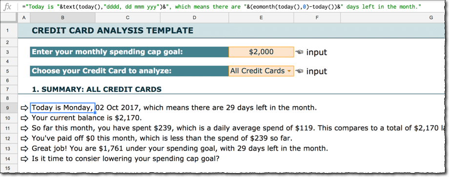
Rather than forcing me to interpret numbers and estimate what's happening, I merely read. The words provide all the context and then I know exactly what'due south happening this month versus final and where I am spend-wise.

These formulas are not conceptually difficult, only they can be long and verbose when you take several options in an IF argument with a mix of text and formulas.

The manner you create these formulas is to wrap your calculation formulas with the the TEXT formula, which formats your numbers correctly. Then yous combine these with any static text using the ampersand, &.

For instance, hither's one of these formulas:

="You've paid off "&text(E26,"$#,##0")&" this month, which is "&if(E26 > C26,"greater","less")&" than the spend of "&text(C26,"$#,##0")&" so far."

where E6 is the amount I've paid towards my credit menu, and C26 is how much I've spent this month.

Read more than about how to combine text and numbers.

As always, let me know your thoughts or questions in the comments!

---

Annotation one: I'thou not a fiscal expert and this postal service does not provide financial advice. It simply shows some techniques for working with and presenting data in Google Sheets.

Note 2: Some of the links in this post are chapter links, meaning I'll go a modest commission if you click the link and after signup to use that vendor'southward service. I only do this for tools I use myself and wholeheartedly recommend.

Source: https://www.benlcollins.com/spreadsheets/google-sheets-budget-template/

Share this post